前回の続きです。
春のパン祭り点数集計を進めていきます。
方針再検討
前回の結果を振り返りつつ、改めて方式を検討します。
前回の状況
- Hue画像での2値化から、シール領域の輪郭取得を実施した
- シールの重なりにより、輪郭どうしがつながってしまっていた
輪郭がつながってしまった件について、Watershedアルゴリズムも考えていましたが、参考サイトを見ると、まずシール領域の中心付近の領域を取得して、そこから領域を広げていきながら境界を見つける、という処理のよう。

前回の画像を見ると、収縮処理や距離変換でシール領域の中心を見つけるのは難しそう。
ということでWatershedアルゴリズムもやってみたかったけど諦めます。
ただ、この2値化画像の最外周輪郭を見ると、全てのシールが内側に含まれていて、この内側の輪郭で点数文字が取得できそうに思えます。
点数文字を取得したら、そこからテンプレートマッチングで点数を識別します。
これを進めてみたいと思います。
台紙やシールの外形によるスケーリング、変形も考えていましたが、これは諦めで。
下準備
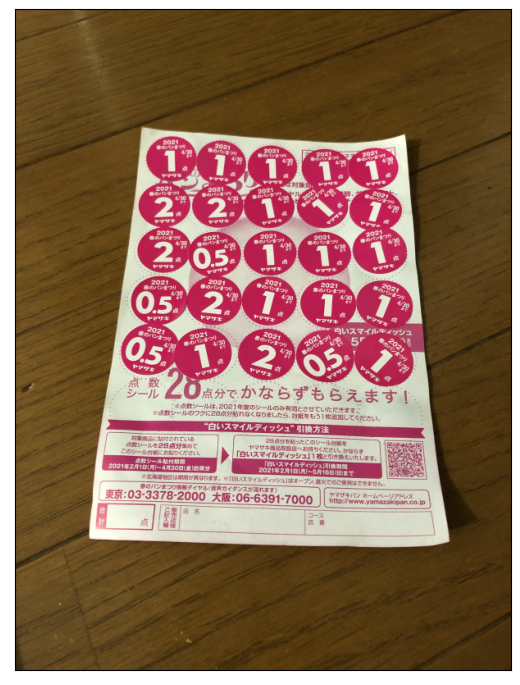
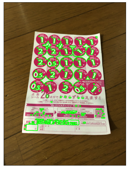
まずはいつもの下準備から。前回の5番目画像だけでやります。
※今回、cv2.resize()での縮小率を0.1から0.2に変更しています。
元の縮小率で進めていましたが、うまくいかなかったりしたので。
あまり大きくすると処理が重くなりそうですが、適度な解像度がありそうです。
import cv2
import numpy as np
%matplotlib inline
from matplotlib import pyplot as plt

img5 = cv2.imread('harupan_210402_1.jpg')
img5 = cv2.resize(img5, None, fx=0.2, fy=0.2, interpolation=cv2.INTER_AREA)
print(img5.shape)
(806, 605, 3)
plt.figure(figsize=(6.4,100), dpi=100)
plt.imshow(cv2.cvtColor(img5, cv2.COLOR_BGR2RGB)), plt.xticks([]), plt.yticks([])
plt.show()
輪郭取得
輪郭を取得しますが、輪郭の階層を利用します。
cv2.findContour()関数では、輪郭取得のモード指定で、輪郭の階層構造も一緒に取得できます。
https://docs.opencv.org/4.5.2/d9/d8b/tutorial_py_contours_hierarchy.html
前回はcv2.RETR_EXTERNALを指定したので最外周輪郭のみ取得になりましたが、cv2.RETR_TREEであれば全輪郭と全階層構造を取得できます。
階層構造は、(1,輪郭の数,4)の形状のndarrayとして得られて、1輪郭あたりの情報としては[Next, Previous, First_Child, Parent]という形で輪郭のインデックスが入ってきます。該当する輪郭がなければ-1が入ります。
- Next: 同じ階層の次の輪郭
- Previous: 同じ階層の前の輪郭
- First_Child: 一つ下の階層の1番目の輪郭
- Parent: 1つ上の階層の輪郭
全輪郭の取得、表示
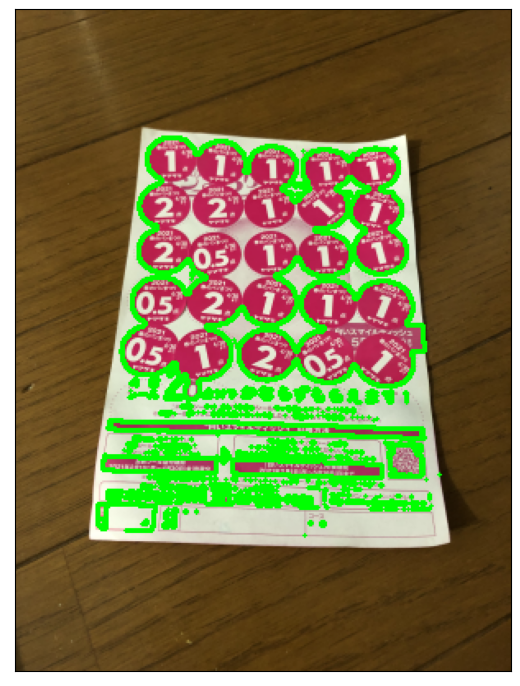
まず全輪郭を見てみて、点数文字の輪郭が取れていそうか確認します。
img5_hsv = cv2.cvtColor(img5, cv2.COLOR_BGR2HSV)
ret, img5_th_hue = cv2.threshold(img5_hsv[:,:,0], 135, 255, cv2.THRESH_BINARY)
img5_contours, img5_hierarchy = cv2.findContours(img5_th_hue, cv2.RETR_TREE, cv2.CHAIN_APPROX_SIMPLE)

img5_with_contours = cv2.drawContours(img5.copy(), img5_contours, -1, (0,255,0), 2)
plt.figure(figsize=(6.4,100), dpi=100)
plt.imshow(cv2.cvtColor(img5_with_contours, cv2.COLOR_BGR2RGB)), plt.xticks([]), plt.yticks([])
plt.show()

print('Shape: ', img5_hierarchy.shape, '\nContents: \n', img5_hierarchy[0,0:20,:], ' ...')
Shape:  (1, 1618, 4)
Contents:
 [[ 1 -1 -1 -1]
 [ 2  0 -1 -1]
 [ 3  1 -1 -1]
 [ 4  2 -1 -1]
 [ 5  3 -1 -1]
 [ 6  4 -1 -1]
 [ 7  5 -1 -1]
 [ 8  6 -1 -1]
 [ 9  7 -1 -1]
 [10  8 -1 -1]
 [11  9 -1 -1]
 [12 10 -1 -1]
 [13 11 -1 -1]
 [14 12 -1 -1]
 [15 13 -1 -1]
 [16 14 -1 -1]
 [17 15 -1 -1]
 [18 16 -1 -1]
 [19 17 -1 -1]
 [20 18 -1 -1]]  ...
大丈夫そうです。
輪郭を階層ごとに分ける
最外周輪郭は、Parentが-1になっている輪郭、ということで探せます。そしてもう1つ下の階層の輪郭は、最外周輪郭をParentとする輪郭、ということで探せます。
img5_indices_level0 = [i for i,hier in enumerate(img5_hierarchy[0,:,:]) if hier[3] == -1]
img5_contours_level0 = [img5_contours[i] for i in img5_indices_level0]
img5_hierarchy_level0 = [img5_hierarchy[0,i,:] for i in img5_indices_level0]
print('Contours Level0')
print('  Number of contours: ', len(img5_hierarchy_level0))
print('  Indices: ', img5_indices_level0[0:min(100,len(img5_indices_level0))], ' ...')
print('  Contents:')
[print(img5_hierarchy_level0[i]) for i in range(20)];
print('...')
Contours Level0
  Number of contours:  499
  Indices:  [0, 1, 2, 3, 4, 5, 6, 7, 8, 9, 10, 11, 12, 13, 14, 15, 16, 17, 18, 19, 20, 21, 22, 23, 24, 25, 26, 27, 28, 30, 31, 32, 33, 34, 35, 36, 37, 38, 39, 40, 41, 42, 43, 44, 45, 46, 47, 48, 49, 50, 51, 52, 53, 54, 55, 56, 64, 66, 68, 70, 72, 73, 74, 75, 76, 79, 80, 81, 82, 83, 84, 85, 87, 90, 91, 92, 93, 94, 95, 96, 97, 98, 99, 100, 103, 104, 105, 106, 107, 108, 109, 110, 111, 112, 113, 118, 119, 120, 123, 124]  ...
  Contents:
[ 1 -1 -1 -1]
[ 2  0 -1 -1]
[ 3  1 -1 -1]
[ 4  2 -1 -1]
[ 5  3 -1 -1]
[ 6  4 -1 -1]
[ 7  5 -1 -1]
[ 8  6 -1 -1]
[ 9  7 -1 -1]
[10  8 -1 -1]
[11  9 -1 -1]
[12 10 -1 -1]
[13 11 -1 -1]
[14 12 -1 -1]
[15 13 -1 -1]
[16 14 -1 -1]
[17 15 -1 -1]
[18 16 -1 -1]
[19 17 -1 -1]
[20 18 -1 -1]
...
img5_indices_level1 = [i for i,hier in enumerate(img5_hierarchy[0,:,:]) if hier[3] in img5_indices_level0]
img5_contours_level1 = [img5_contours[i] for i in img5_indices_level1]
img5_hierarchy_level1 = [img5_hierarchy[0,i,:] for i in img5_indices_level1]
print('Contours Level1')
print('  Number of contours: ', len(img5_hierarchy_level1))
print('  Indices: ', img5_indices_level1[0:min(100,len(img5_indices_level1))], ' ...')
print('  Contents:')
[print(img5_hierarchy_level1[i]) for i in range(20)];
print('...')
Contours Level1
  Number of contours:  1094
  Indices:  [29, 57, 58, 60, 65, 67, 69, 71, 77, 78, 86, 88, 89, 101, 102, 114, 115, 116, 117, 121, 122, 125, 128, 129, 135, 137, 138, 147, 169, 170, 183, 184, 226, 227, 228, 253, 268, 269, 270, 271, 272, 273, 274, 275, 276, 277, 278, 279, 280, 281, 282, 283, 284, 285, 286, 287, 288, 289, 292, 293, 294, 295, 296, 297, 298, 299, 300, 301, 302, 303, 304, 305, 306, 307, 308, 309, 310, 311, 312, 321, 322, 339, 354, 358, 364, 381, 382, 384, 388, 389, 390, 391, 392, 393, 394, 395, 396, 397, 398, 399]  ...
  Contents:
[-1 -1 -1 28]
[58 -1 -1 56]
[60 57 59 56]
[-1 58 61 56]
[-1 -1 -1 64]
[-1 -1 -1 66]
[-1 -1 -1 68]
[-1 -1 -1 70]
[78 -1 -1 76]
[-1 77 -1 76]
[-1 -1 -1 85]
[89 -1 -1 87]
[-1 88 -1 87]
[102  -1  -1 100]
[ -1 101  -1 100]
[115  -1  -1 113]
[116 114  -1 113]
[117 115  -1 113]
[ -1 116  -1 113]
[122  -1  -1 120]
...
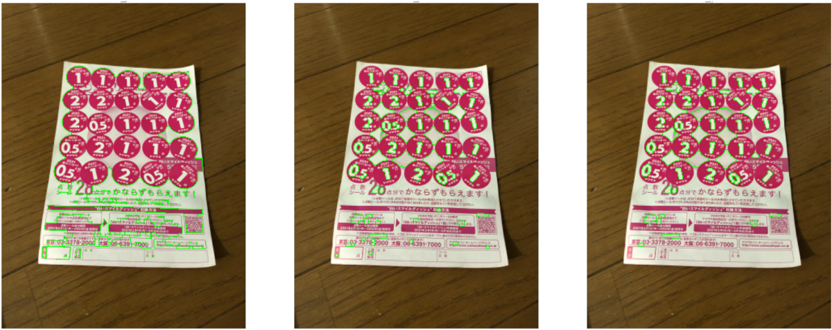
img5_with_contours0 = cv2.drawContours(img5.copy(), img5_contours_level0, -1, (0,255,0), 2)
img5_with_contours1 = cv2.drawContours(img5.copy(), img5_contours_level1, -1, (0,255,0), 2)
plt.figure(figsize=(6.4,100), dpi=100)
plt.subplot(121), plt.imshow(cv2.cvtColor(img5_with_contours0, cv2.COLOR_BGR2RGB)), plt.title('Level0'), plt.xticks([]), plt.yticks([])
plt.subplot(122), plt.imshow(cv2.cvtColor(img5_with_contours1, cv2.COLOR_BGR2RGB)), plt.title('Level1'), plt.xticks([]), plt.yticks([])
plt.show()
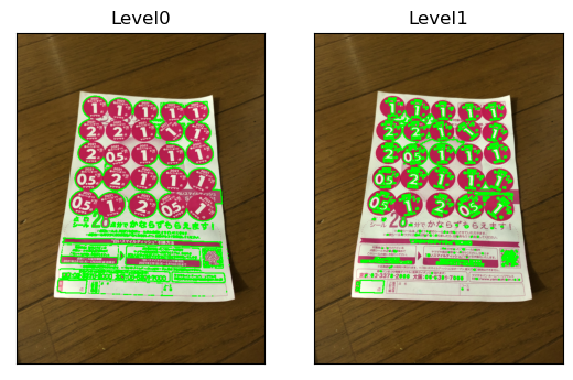
それらしい感じになりました。
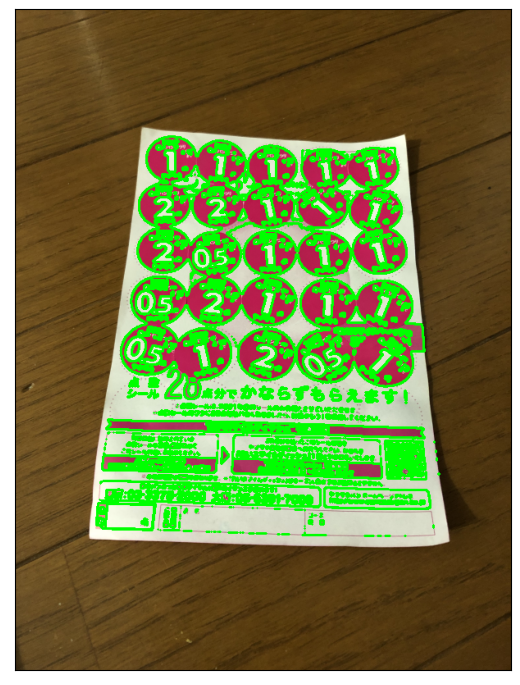
モルフォロジー変換での2値化画像の調整
Level1の輪郭を見ると、細かい文字の部分の輪郭も取ってしまっているように見えます。
2値化の後にモルフォロジー変換のClosing処理(収縮→膨張)をやってから輪郭検出してみます。
kernel = np.ones((3,3),np.uint8)
img5_th_hue2 = cv2.morphologyEx(img5_th_hue, cv2.MORPH_CLOSE, kernel)
img5_contours, img5_hierarchy = cv2.findContours(img5_th_hue2, cv2.RETR_TREE, cv2.CHAIN_APPROX_SIMPLE)

img5_indices_level0 = [i for i,hier in enumerate(img5_hierarchy[0,:,:]) if hier[3] == -1]
img5_contours_level0 = [img5_contours[i] for i in img5_indices_level0]
img5_hierarchy_level0 = [img5_hierarchy[0,i,:] for i in img5_indices_level0]
img5_indices_level1 = [i for i,hier in enumerate(img5_hierarchy[0,:,:]) if hier[3] in img5_indices_level0]
img5_contours_level1 = [img5_contours[i] for i in img5_indices_level1]
img5_hierarchy_level1 = [img5_hierarchy[0,i,:] for i in img5_indices_level1]

img5_with_contours0 = cv2.drawContours(img5.copy(), img5_contours_level0, -1, (0,255,0), 2)
img5_with_contours1 = cv2.drawContours(img5.copy(), img5_contours_level1, -1, (0,255,0), 2)
plt.figure(figsize=(6.4,100), dpi=100)
plt.imshow(cv2.cvtColor(img5_with_contours1, cv2.COLOR_BGR2RGB)), plt.xticks([]), plt.yticks([])
plt.show()
いい感じになってきました。
輪郭面積によるフィルタリング
ついでに、極端に小さい面積の輪郭は除去したほうがいいのかなと。
面積のヒストグラムを見てみます。
img5_areas_level1 = [cv2.contourArea(ctr) for ctr in img5_contours_level1]
plt.hist(img5_areas_level1, 100)
plt.show()
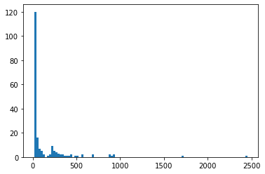
小さい面積の部分を拡大してみると、
plt.hist(img5_areas_level1, 100, [0,500])
plt.show()
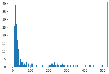
面積100pixel分を閾値としてやってみます。
100pixelというと、10x10pixelぐらいの領域ですが、今回の画像は800x600ピクセルぐらいだったので、画像全体に対して縦1/80、横1/60ぐらい→画像全体の面積の1/4800のサイズになります。
それに対して、点数文字の大きさをかなりおおざっぱに
- シール台紙が画像全体の縦横半分程度は写っているとする (写るようにする)
- シールが縦横に5個ずつ並んでいる
- 点数文字はシールのおよそ縦横半分程度の大きさはある
と考えると、画像全体に対してだいたい縦横1/20ぐらい→画像全体の面積の1/400程度のサイズとなります。
今回の画像でいうと、1000pixelぐらいになる?
ヒストグラムを見ると、200~500pixelあたりの面積の輪郭が点数文字に当たるかと。誤差は大きいですが、およそスケール感としてはそんなところかと。
画像全体の1/4000ぐらいを閾値とするのでいいかと思います。
img5_contours_level1_2 = [ctr for ctr in img5_contours_level1 if cv2.contourArea(ctr) > 100]
img5_with_contours1 = cv2.drawContours(img5.copy(), img5_contours_level1_2, -1, (0,255,0), 2)
plt.figure(figsize=(6.4,100), dpi=100)
plt.imshow(cv2.cvtColor(img5_with_contours1, cv2.COLOR_BGR2RGB)), plt.title('Level1'), plt.xticks([]), plt.yticks([])
plt.show()
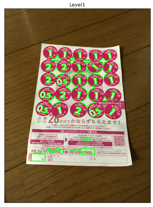
よりいい感じになってきました。
今回はここまで
少し違うものも混ざってしまっていますが、およそいい感じに点数文字の輪郭が取れました。
次回はここから点数文字のテンプレートマッチングをやっていきたいと思います。
ついでに
一応元の縮小率(0.1)での結果を出しておきます。
輪郭面積でのフィルタリングのとき、面積の閾値は、縮小率が2倍になっていることを考慮して、上での閾値の1/4 -> 25とします。
img5_01 = cv2.imread('harupan_210402_1.jpg')
img5_01 = cv2.resize(img5_01, None, fx=0.1, fy=0.1, interpolation=cv2.INTER_AREA)
img5_01_hsv = cv2.cvtColor(img5_01, cv2.COLOR_BGR2HSV)
ret, img5_01_th_hue = cv2.threshold(img5_01_hsv[:,:,0], 135, 255, cv2.THRESH_BINARY)
img5_01_th_hue = cv2.morphologyEx(img5_01_th_hue, cv2.MORPH_CLOSE, kernel)
img5_01_contours, img5_01_hierarchy = cv2.findContours(img5_01_th_hue, cv2.RETR_TREE, cv2.CHAIN_APPROX_SIMPLE)
img5_01_indices_level0 = [i for i,hier in enumerate(img5_01_hierarchy[0,:,:]) if hier[3] == -1]
img5_01_contours_level0 = [img5_01_contours[i] for i in img5_01_indices_level0]
img5_01_indices_level1 = [i for i,hier in enumerate(img5_01_hierarchy[0,:,:]) if hier[3] in img5_01_indices_level0]
img5_01_contours_level1 = [img5_01_contours[i] for i in img5_01_indices_level1]
img5_01_contours_level1_2 = [ctr for ctr in img5_01_contours_level1 if cv2.contourArea(ctr) > 25]
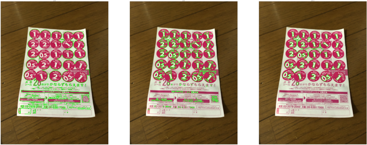
img5_01_with_contours1_2 = cv2.drawContours(img5_01.copy(), img5_01_contours_level1_2, -1, (0,255,0), 2)
img5_01_with_contours0 = cv2.drawContours(img5_01.copy(), img5_01_contours_level0, -1, (0,255,0), 1)
img5_01_with_contours1 = cv2.drawContours(img5_01.copy(), img5_01_contours_level1, -1, (0,255,0), 1)
img5_01_with_contours1_2 = cv2.drawContours(img5_01.copy(), img5_01_contours_level1_2, -1, (0,255,0), 1)
plt.figure(figsize=(100,100), dpi=100)
plt.subplot(131), plt.imshow(cv2.cvtColor(img5_01_with_contours0, cv2.COLOR_BGR2RGB)), plt.title('Level0'), plt.xticks([]), plt.yticks([])
plt.subplot(132), plt.imshow(cv2.cvtColor(img5_01_with_contours1, cv2.COLOR_BGR2RGB)), plt.title('Level1'), plt.xticks([]), plt.yticks([])
plt.subplot(133), plt.imshow(cv2.cvtColor(img5_01_with_contours1_2, cv2.COLOR_BGR2RGB)), plt.title('Level1_2'), plt.xticks([]), plt.yticks([])
plt.show()
こちらでは、2や5の文字輪郭がうまく取得できませんでした。
ただ、この後試しにモルフォロジー変換なしでやってみると、
ret, img5_01_th_hue = cv2.threshold(img5_01_hsv[:,:,0], 135, 255, cv2.THRESH_BINARY)
img5_01_contours, img5_01_hierarchy = cv2.findContours(img5_01_th_hue, cv2.RETR_TREE, cv2.CHAIN_APPROX_SIMPLE)
img5_01_indices_level0 = [i for i,hier in enumerate(img5_01_hierarchy[0,:,:]) if hier[3] == -1]
img5_01_contours_level0 = [img5_01_contours[i] for i in img5_01_indices_level0]
img5_01_indices_level1 = [i for i,hier in enumerate(img5_01_hierarchy[0,:,:]) if hier[3] in img5_01_indices_level0]
img5_01_contours_level1 = [img5_01_contours[i] for i in img5_01_indices_level1]
img5_01_contours_level1_2 = [ctr for ctr in img5_01_contours_level1 if cv2.contourArea(ctr) > 25]
img5_01_with_contours1_2 = cv2.drawContours(img5_01.copy(), img5_01_contours_level1_2, -1, (0,255,0), 2)
img5_01_with_contours0 = cv2.drawContours(img5_01.copy(), img5_01_contours_level0, -1, (0,255,0), 1)
img5_01_with_contours1 = cv2.drawContours(img5_01.copy(), img5_01_contours_level1, -1, (0,255,0), 1)
img5_01_with_contours1_2 = cv2.drawContours(img5_01.copy(), img5_01_contours_level1_2, -1, (0,255,0), 1)
plt.figure(figsize=(100,100), dpi=100)
plt.subplot(131), plt.imshow(cv2.cvtColor(img5_01_with_contours0, cv2.COLOR_BGR2RGB)), plt.title('Level0'), plt.xticks([]), plt.yticks([])
plt.subplot(132), plt.imshow(cv2.cvtColor(img5_01_with_contours1, cv2.COLOR_BGR2RGB)), plt.title('Level1'), plt.xticks([]), plt.yticks([])
plt.subplot(133), plt.imshow(cv2.cvtColor(img5_01_with_contours1_2, cv2.COLOR_BGR2RGB)), plt.title('Level1_2'), plt.xticks([]), plt.yticks([])
plt.show()
という感じで、縮小率を変える前と同様の輪郭が取れました。
- 縮小率の高い画像にとっては3x3のカーネルが大き過ぎた
- 輪郭面積でのフィルタリングでも、結果的にモルフォロジー変換を適用したのと同じ結果が得られる
ということかと思います。
ただ、縮小率0.2での輪郭に比べると、解像度不足からぎざぎざしてしまっている感じがするので、やっぱり縮小率0.2で進めていきたいと思います。
検出対象の画像データ中の大きさを意識しておく必要がる、ということかと思います。


